Hénon Map MATLAB

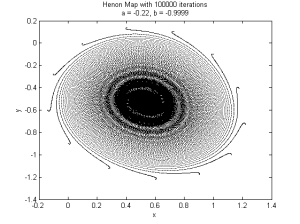
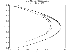
In my studying of dynamical systems I stumbled upon the Hénon Map today, a two-dimensional dynamical system with a strange attractor which demonstrates chaotic behaviour. The system is described by a coupled pair of equations. Here’s what the classical version looks like:

The classical Hénon Map.

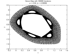
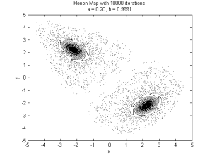
There are only two parameters, but playing around with them yields some interesting results:

A variation of the Hénon Map

Another variation of the Hénon Map

Yet another variation of the Hénon Map

Again, the code to implement this is pretty simple, so I’ll post it here as opposed to GitHub (though I’ll probably post a version on GitHub which draws the system state after each iteration):

a = 1.4;
b = 0.3;
iterations = 10000;
x = zeros(1, iterations);
y = zeros(1, iterations);
% simulation
for i=1:iterations
x(1,i+1) = 1-(a*x(1,i)^2) + y(1,i);
y(1,i+1) = b*x(1,i);
end
% plotting
plot(x(5:iterations),y(5:iterations), '.k','MarkerSize',3)
line1 = sprintf('Henon Map with %.0f iterations', iterations);
line2 = sprintf('a = %.2f, b = %.5f', a, b);
title({line1, line2});
xlabel('x')
ylabel('y')


Liapunov plot in MATLAB

I seem to do a lot of MATLAB coding… In a paper I’m studying I came across the following:

“… in which case it is a dissipative system possessing a Liapunov function … thus, released from an initial (non-equilibrium) state, typical solutions approach asymptotically stable fixed points (sinks).”

(Brown & Holmes (2001), Modelling a simple choice task: Stochastic dynamics of mutually inhibitory neural groups, Stochastics  and Dynamics, 1:2 (2001), 159-191))

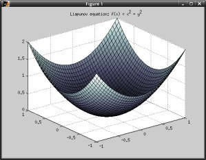
So I’ve been doing a bit of background reading on system stability (in linear systems) and Liapunov functions, which can be used to prove the stability of an equilibrium of an ordinary differential equation. I plotted a simple one in MATLAB:

Plot of a simple Liapunov function

There isn’t really a lot of code behind it, so I’ll just post it here (I also might update this later with slightly more complicated functions):

x = [-1:.05:1];
y = x;
[x,y] = meshgrid(x,y);
z = x.^2 + y.^2;
figure(1)
colormap(bone)
surf(x,y,z)
title('Liapunov equation: f(x) = x^2 + y^2')

Lotka-Volterra MATLAB model

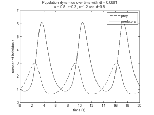
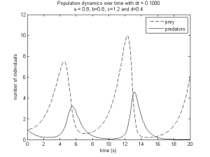
I’m starting to play with dynamical systems so I figured I’d post a baby model. It essentially shows the growth of two populations co-existing together, one being the prey, the other the predators. A small time step (dt) shows that the system is stable; a larger one leads to instability and thus highlights the importance of parameter choice.

Small dt example (populations oscillate in a stable manner):

Population growth with small changes in time.

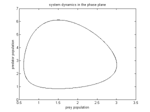
Plotting the two populations in the phase plane yields this:

Phase plane for the system.

Large dt example, where the population growth is without bounds:

Population growth with large changes in time.

Plotting the two populations in the phase plane yields something quite different:

Phase plane for the system.

As always, the code is over on my GitHub.

Drift Diffusion MATLAB Model

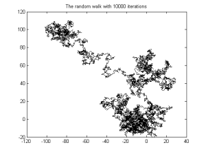
Just spent a good eight/nine hours redesigning my website from the ground up. I’m happy with the result (for a few months at least), so figured I’d take a little break and make a blog entry. I finally got round to implementing the drift diffusion model a few weeks back, one of the classical models of decision making. This is essentially the random walker with a bias, or “drift” towards one of the choices (in a two alternative forced choice task). This is one of the results from a simulation:

Drift diffusion model implemented in MATLAB.

As always, the code that produced this is available over at my GitHub. I’ll be attempting the pooled inhibition model shortly, as well as investigating some more focused behavioural experiments with honeybees and drosophila. 

Random Walker MATLAB

In reading about optimal decision making I came across the drift diffusion model; an integrator that demonstrates “random walk” behaviour. So I figured I’d implement a 2D random walker in MATLAB.

This is the result:

Output of the Random Walker simulation.

The code that produced this is over at my GitHub.

leaky integrate and fire MATLAB model

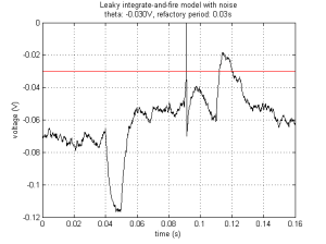
LIF is considered as one of the simpler spiking neuron models, and I’ve been doing a bit of work with it in MATLAB:

Leaky intergrate-and-fire graph

The graph shows the membrane potential of a neuron over time. There’s an inhibitory current injection at 0.04 seconds, followed by an excitatory injection at 0.05 and 0.09 seconds. The second current injection causes the voltage to exceed a set threshold (shown by the red line), and so an activation potential is generated (the neuron spikes). A final excitatory injection is given at 0.11 seconds, however this is within the time of the absolute refractory period: although the voltage crosses the threshold again, the neuron doesn’t spike.

The code is over on my GitHub.

Feng, J. (2001). Is the integrate-and-fire model good enough?–a review. Neural networks : the official journal of the International Neural Network Society, 14(6-7), 955–75.